What is VLOOKUP in Excel?
VLOOKUP is a built-in Excel function used to search for a value in the first column of a table range and return a corresponding value from another column in the same row. It stands for “Vertical Lookup” and is commonly used for data retrieval and analysis tasks.
Limitations of VLOOKUP in Excel
Here are some limitations of VLOOKUP in Excel:
- VLOOKUP only looks for a match in the first column of the lookup range. This means you cannot use it to search for a value in a different column of the lookup range.
- VLOOKUP is not case-sensitive, so it may return incorrect results if the lookup value is in a different case than the data in the lookup range.
- VLOOKUP only returns the first matching value in the lookup range. This means that if there are multiple occurrences of the lookup value in the lookup range, VLOOKUP will only return the first one.
- VLOOKUP can only handle data that is sorted in ascending order. This means that if the data is not sorted, VLOOKUP may return an incorrect result.
- VLOOKUP cannot handle data that contains errors or blank cells. If the lookup range contains errors or blank cells, VLOOKUP may return an incorrect result.
- VLOOKUP is not very flexible when changing the lookup value or range. If you need to change the lookup value or the lookup range, you must manually update the VLOOKUP formula
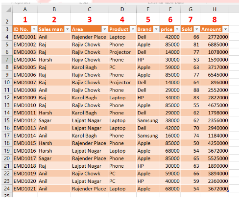
Step 1: Create Database check below picture…
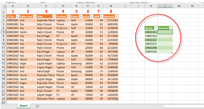
Step 2: Create Vertical lookup index below picture…
Step 3: Use Vlookup Formula check below picture

Formula Selection Steps
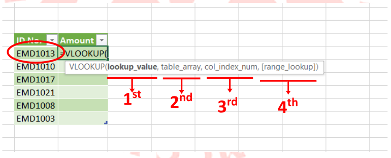
1st Selection: – select individual ID show on left of formula
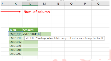
2nd Selection: – Select Whole data table where from you View result
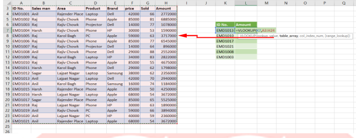
3rd Selection: – Type Column position what you want to show in Result cell. Check below picture

4th Selection: – “FALSE” if you want exact value/ “TRUE” if you want approximate value.
TRUE in num. form (1)
FASLE in Num. form (0)
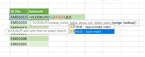
Done.


I’m extremely impressed with your writing abilities as well as with the structure to
your weblog. Is this a paid subject matter or did you customize it
yourself? Either way keep up the excellent quality writing, it’s uncommon to
see a great weblog like this one these days. Snipfeed!