
HLOOKUP is an Excel function to looks up and retrieves data from a specific row in a table. It searches for a value in the table’s first row and returns another value in the same column from a row according to the given condition.
The HLOOKUP function is used to search for a value in the top row of an array of values, and then it retrieves the value in the same column from a row you specify in the table or array. The H in HLOOKUP stands for ‘Horizontal ‘. In this article, we will help you understand how to use the HLOOKUP function along with the example.
Difference Between VLOOKUP and HLOOKUP?
The VLOOKUP function is used to look up a particular value in a table array organized vertically and then return data from a specified column against that value.
Whereas, we use the HLOOKUP to look up a value horizontally. This is done by searching the top row of the table for a specified value and in return giving back the value in the same column.
How to use HLOOKUP?
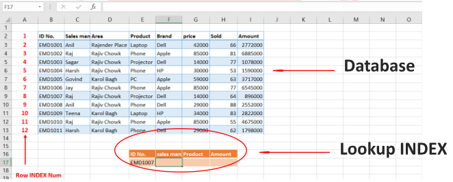
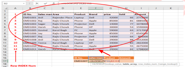
Step 1: Create Database & Lookup index table
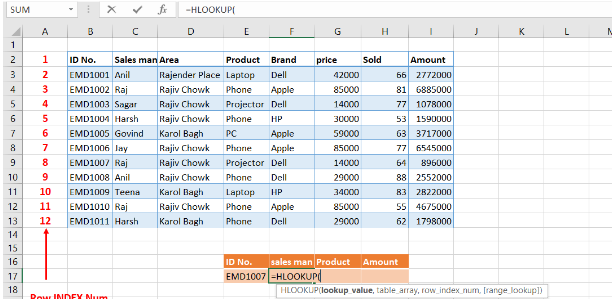
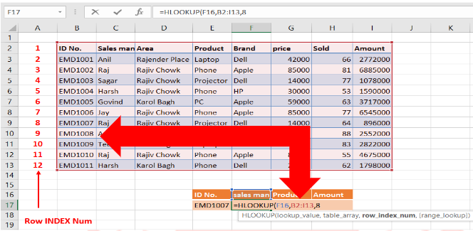
Step 2: Use the Hlookup formula to find the value
Formula selection Steps
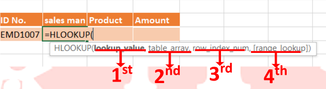
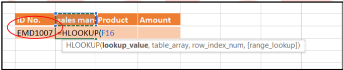
1st Step: select ID num. which emp. Info. you want to check
2nd Step: Select database tale for find your result
3rd Step: Type ROW INDEX num. Which row ID do you want to find for your result value?
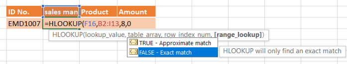
4th Step: “FALSE” if you want exact value/ “TRUE” if you want approximate value.
TRUE in num. form (1)
FASLE in Num. form (0)
Final Result
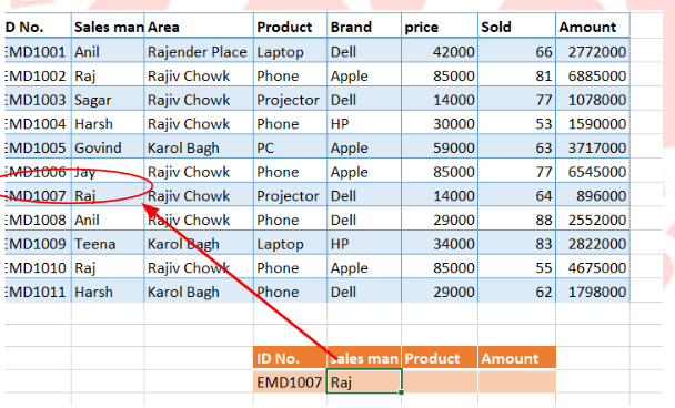
Done.