What are pivot tables used for?
The purpose of pivot tables is to offer user-friendly ways to quickly summarize large amounts of data. They can be used to better understand, display, and analyse numerical data in detail.
With this information, you can help identify and answer unanticipated questions surrounding the data.
Here are five hypothetical scenarios where a pivot table could be helpful.
- Comparing Sales Totals of Different Products
- Showing Product Sales as Percentages of Total Sales
- Combining Duplicate Data
- Getting an Employee Headcount for Separate Departments
- Adding Default Values to Empty Cells
How to Create a Pivot Table?
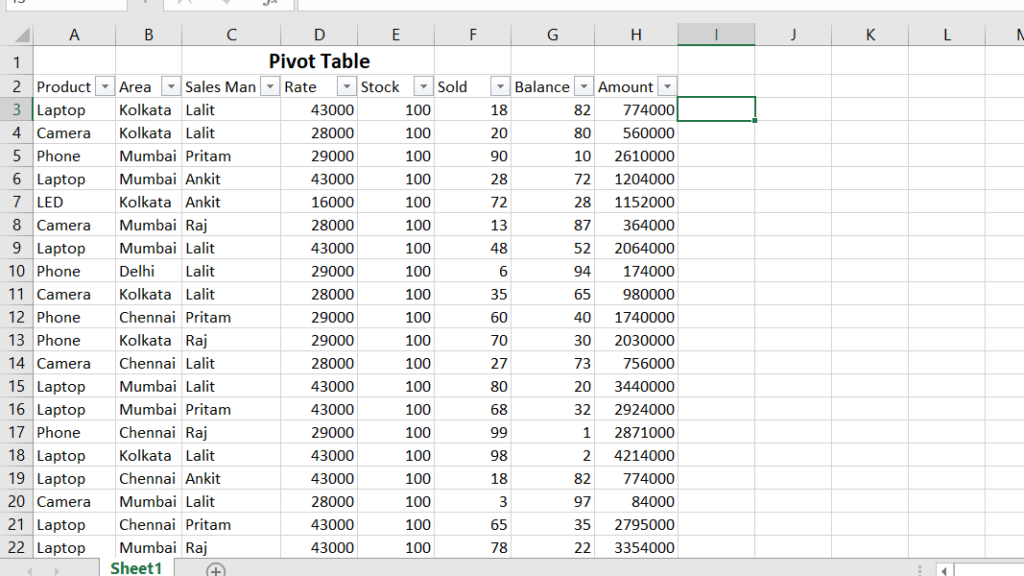
Step 1. Enter your data into a range of rows and columns.
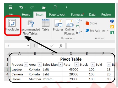
Step 2. Insert your pivot table.
Inserting your pivot table is actually the easiest part. You’ll want to:
- Highlight your data.
- Go to Insert in the top menu.
- Click Pivot table.
A dialog box will come up, confirming the selected data set, it will also ask you where you want to place your pivot table. I recommend using a new worksheet.
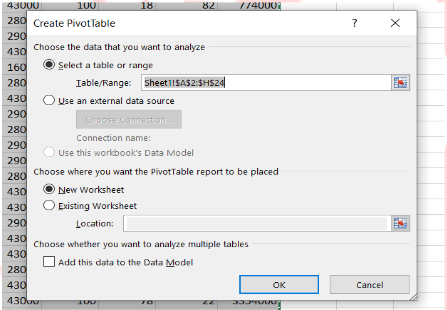
“Once you’ve double-checked everything, click OK.
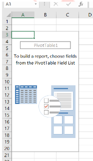
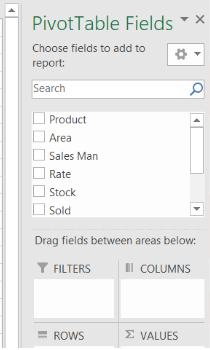
You will then get an empty result like this:
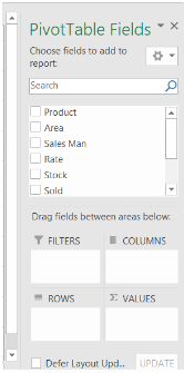
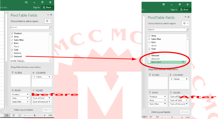
Step 3. Edit your pivot table fields.
Step 4: tick all checkbox … and show below picture…
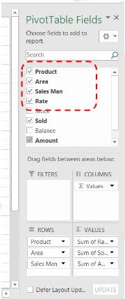
Data will show like this…
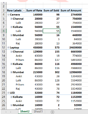
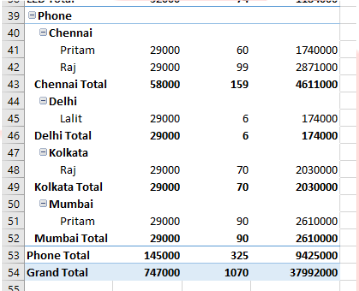
Step 5: The subtotal option is permission to hide and show individual Product Total…
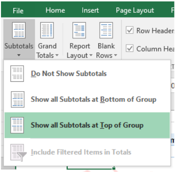
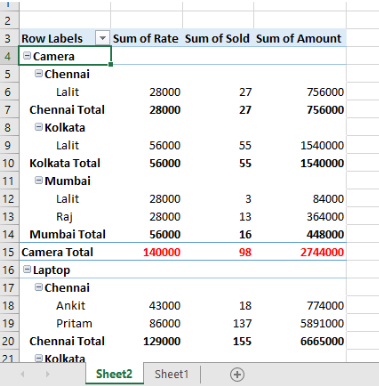
Show in the table …
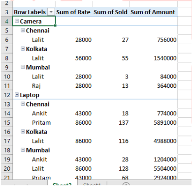
If you want to remove individual total….”Do no show subtotal”
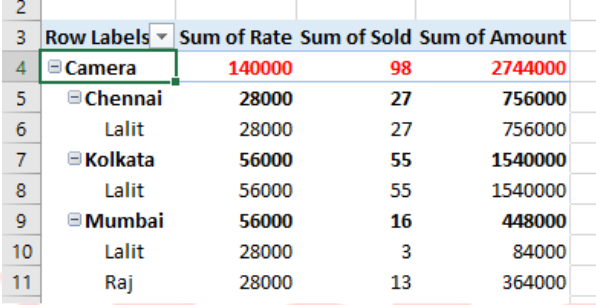
If you show the total at the bottom, click on “show all Subtotals at top of group”
The “grand total” is all data it will show the whole database
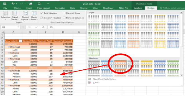
Step 6: Quick format pivot table using “Pivot table” Format.
Refresh (Alt+F5): if you change anything in pivot data you will update all information in the pivot table
Change Data Source: it will be used to add new information to the pivot table
Clear: it will clean all the checkboxes and revert the data same as first view.
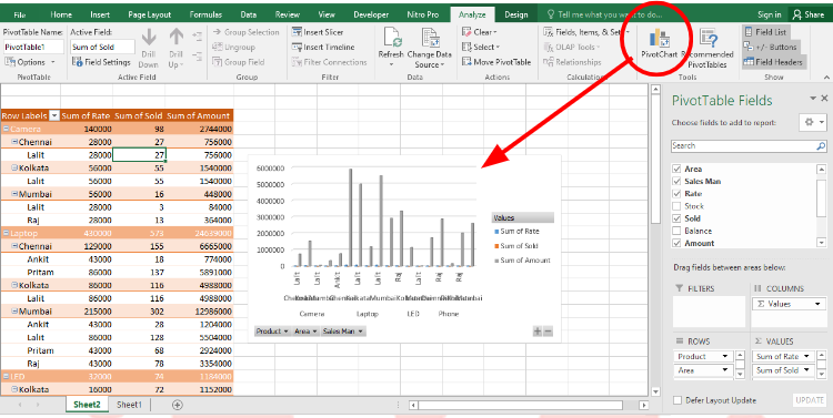
Pivot Chart: Create a chart to represent the pivot table in graph mode.
I was looking at some of your content on this site and I conceive this website is real informative!
Retain putting up.Raise your business